Pythonで感情分析を勉強する

VBAを使った簡単なプログラミングしか経験がない初心者が、Pythonを使った機械学習に挑戦してみることにしました。
機械学習を始めたばかりで、間違いが多くあるかもしれませんが、温かい目で見ていただき、おかしな点があればどうぞご指摘ください。

実行環境

・Python 3.10.12
・Google Colaboratory　（CPU/GPU）

使用したデータ

・Kaggle(Tweet Sentiment Extraction)
Tweet Sentiment Extraction | Kaggle

どのようなデータなのか

ツイートの内容を、
・ネガティブ
・ポジティブ
・ニュートラル
に分類をしたデータです。
このデータを使い、これから入力をするテキストが何に分類されるのかを調べる分類モデルを作成しようと思います。
まずデータについて調べます。

データの中身と個数

import numpy as np
import pandas as pd
#データの読み込み
df = pd.read_csv('/content/train.csv')

#ファイルの中身を確認
print('-' * 10 + 'train' + '-' * 10)
display(df.head()) 
display(df.describe())
display(df.groupby('sentiment').count())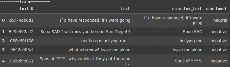

実行結果　display(df.head())

先頭から5行を出力しました。
textID, text, selected_text, sentimentの4列が存在することがわかります。
※今回textID,selected_textは使用しません。

実行結果　display(df.describe())

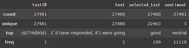
各列の要約統計量を出力しました。
・count = 要素の個数
・unique = ユニークの個数
textIDは27481に対して、textが27480となっています。
どうやら1行だけtextが空になっているようです。

実行結果　display(df.groupby('sentiment').count())

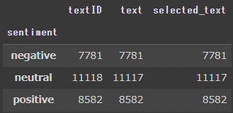
sentimentをグループ化し、データがいくつあるのかを調べます。
合計数は27481ですが、sentimentに偏りがあることがわかりました。

RNNを使い感情分析をする

不要な文字の削除

文章に頻繁に現れるストップワード（I,What,to等）を削除し、分析に必要な単語だけになるよう処理をします。
新たにclean_text列を作成し、その中に処理後の文章を格納します。

import numpy as np
import pandas as pd

#データの読み込み
df = pd.read_csv('/content/train.csv')

#空行の削除
df.dropna(inplace=True)

#不要な列の削除
df = df.drop(['textID','selected_text'],axis = 1)
df = df.reset_index(drop=True)

import re
import nltk
from nltk.corpus import stopwords

#ストップワードの読み込み
nltk.download('stopwords')

#データの前処理関数
def tweet_to_words(raw):

    text = raw.lower()#小文字にする
    text = re.sub("https?://\S+|www\.\S+","",text)#URLを削除
    text = re.sub("\n","",text)#改行を削除
    text = re.sub("[^a-zA-Z@]"," ",text)#文字以外を空白
    words = text.split()#単語のリストを作成
    
    #ストップワードの削除
    stops = set(stopwords.words("english"))
    clean_words = [w for w in words if not w in stops and not re.match('^[@]',w)]
    return " ".join(clean_words)

# データの前処理
df['clean_text'] = df['text'].apply(lambda x:tweet_to_words(x))

処理前：「Why does my boss have to come in today.....」
処理後：「boss come today」
このようにデータがコンパクトになりました。

データの前処理

学習モデルで読み込みできるよう文章の前処理をします。
前処理の手順は以下です。
・感情に影響を与える単語を調べるために、単語の辞書を作成し出現頻度タグ付けを行う
・辞書を使って単語を数値化する
・データのサイズを統一する
次にネガティブ・ポジティブ・ニュートラルの感情ラベルを数値化し、モデルに適した形式に変換します。

#各単語の出現回数を格納
from collections import Counter
counts = Counter([word for clean in df['clean_text'] for word in clean.split()])

#降順に並び替えをします。
vocab = sorted(counts,key=counts.get,reverse=True)
vocab_to_list = {word:i for i,word in enumerate(vocab,1)}

#文字列を数値化したリストを作成する
vocab_ints = []
for each in df['clean_text']:
    vocab_ints.append([vocab_to_list[word] for word in each.split()])
    
#文章ごとのネガポジ評価を数値化
sentiment_labels = np.array([0 if each == 'negative' else 1 if each == 'positive' else 2 for each in df['sentiment']])

#vocab_ints内の最大文字数を格納
vocab_len = Counter([len(x) for x in vocab_ints])
seq_len = max(vocab_len)

#文章の長さが0でない行を選択
tweet_idx = [idx for idx,word in enumerate(vocab_ints) if len(word) > 0]
sentiment_labels = sentiment_labels[tweet_idx]
df = df.iloc[tweet_idx]
vocab_ints = [word for word in vocab_ints if len(word) > 0]

features = np.zeros((len(vocab_ints),seq_len),dtype=int)

#数値化した単語を右からセットする
for i,row in enumerate(vocab_ints):
    features[i,-len(row):] = np.array(row)[:seq_len]

学習データ、感情ラベルの作成

8割を訓練データ、2割を検証データとテストデータに分けます。
その後、データ、感情ラベルをRNNで読み込みできる形式に変換をします。
※先ほど、感情ラベルを数値化しましがこのまま使うことができないので
negative → [1, 0, 0]
positive → [0, 1, 0]
neutral → [0, 0, 1]
このような形になるよう「one-hotベクトル」に変換をします。

# 訓練データ、検証データ、テストデータの作成
train_size = int(len(features)*0.8)
train_x,val_x = features[:train_size],features[train_size:]
train_y,val_y = sentiment_labels[:train_size],sentiment_labels[train_size:]

test_idx = int(len(val_x)*0.5)
val_x, test_x = val_x[:test_idx], val_x[test_idx:]
val_y, test_y = val_y[:test_idx], val_y[test_idx:]

#学習データをＲＮＮで読み込みする(サンプル数, シーケンス長, 次元数) の形に変換する
train_x = np.reshape(train_x,(train_x.shape[0],1, train_x.shape[1]))
val_x =  np.reshape(val_x, (val_x.shape[0], 1, val_x.shape[1]))
test_x=  np.reshape(test_x, (test_x.shape[0], 1, test_x.shape[1]))

from tensorflow.keras.utils import to_categorical

#正解ラベルをonehotベクトルに変換
train_y = to_categorical(train_y, 3)
val_y = to_categorical(val_y, 3)
test_y = to_categorical(test_y,3)

モデルの作成～評価まで

LSTM層を追加したモデルを作成し、コンパイル→学習の実行→モデルの評価をしていきます。

from tensorflow.keras.layers import Dense,Activation,LSTM
from tensorflow.keras.callbacks import EarlyStopping
from tensorflow.keras.models import Sequential

#モデルの作成
lstm_model = Sequential()
lstm_model.add(LSTM(units=60,input_shape=(train_x.shape[1], train_x.shape[2]), return_sequences=True))
lstm_model.add(LSTM(units=30, return_sequences=False))
lstm_model.add(Dense(units=3 , activation='softmax'))

#モデルのコンパイル
lstm_model.compile(optimizer='rmsprop',
              loss='categorical_crossentropy',
              metrics=['accuracy'])

#学習
lstm_model.fit(train_x, train_y, validation_data=(val_x, val_y), epochs=5, batch_size=16)

# テストデータの感情ラベルを予測
predictions = lstm_model.predict(test_x)

# 予測結果を最も確率の高いクラスに変換
predicted_labels = np.argmax(predictions, axis=1)
print(predicted_labels)
print(test_y)

# 正解ラベルと比較して精度を計算
accuracy = np.mean(predicted_labels == np.argmax(test_y, axis=1))

print("テストデータの精度:", accuracy)

学習結果と精度の結果が出力されました。

#訓練中の損失、正確性
Epoch 1/5 1370/1370 [==============================] - 12s 6ms/step - loss: 1.0872 - accuracy: 0.3955 - val_loss: 1.0894 - val_accuracy: 0.3954 
Epoch 2/5 1370/1370 [==============================] - 7s 5ms/step - loss: 1.0837 - accuracy: 0.4009 - val_loss: 1.0903 - val_accuracy: 0.3958 
Epoch 3/5 1370/1370 [==============================] - 8s 6ms/step - loss: 1.0823 - accuracy: 0.4028 - val_loss: 1.0893 - val_accuracy: 0.3976 
Epoch 4/5 1370/1370 [==============================] - 8s 6ms/step - loss: 1.0820 - accuracy: 0.4033 - val_loss: 1.0892 - val_accuracy: 0.3928 
Epoch 5/5 1370/1370 [==============================] - 7s 5ms/step - loss: 1.0822 - accuracy: 0.4040 - val_loss: 1.0885 - val_accuracy: 0.3969
テストデータの精度: 0.4135036496350365

テキストの感情分析

学習結果が悪いですが、このままテキストの感情分析をします。
学習したモデルに新たなテキストを入力します。
入力する際は、学習した形式と同じものに変換をしてから実行をします。

new_text = 'This summer is long! Too hot!'

# 英語textの形態素解析をする。
text = tweet_to_words(new_text)
text = text.split()

# 学習したデータベースにない単語は0にする
words_int = []
for word in text:
    try:
        words_int.append(vocab_to_int[word])
    except :
        words_int.append(0)

# モデルが学習したデータの形に加工して予測する
features = np.zeros((1, seq_len), dtype=int)
features[0][-len(words_int):] = words_int
features = np.reshape(features, (1, features.shape[0], features.shape[1]))
predict = lstm_model.predict([features])
answer = np.argmax(predict)

s_label = ['negative','positive','neutral']
print(f'テキスト：{newl_text}\n形態素解析：{text}\n予測結果：{s_label[answer]}')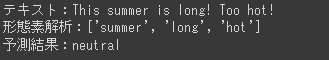

テキストの分析結果

このような結果となりました。
ネガティブだと思ったテキストが、ニュートラルになってしまいました。

反省

期待した結果とは違い、損失が多く、正解率も低いです。
原因として
・文章内に略語が含まれる、スペルの違いが含まれている可能性がある
・各感情ラベル（negative/positive/neutral）の数に偏りがある
 ※データの個数で確認済みです。
以上が考えられます。
その為、学習に偏りがあり上手く感情分析ができない状態となっているようでした。アンダーサンプリングや、ランダムに並び替えをした状態で実行をしましたが同じような結果となりました。
もっと、ノイズの除去やパラメーターの調整のようです。今後の課題としたいと思います。
今回は、別のモデルを使用し分析をすることにしました。

BERTで感情分析をする

BERTは事前学習されたモデルで、様々なことに利用をされています。
文脈を前後両方から考慮し優れた性能を発揮し、感情分析にも優れています。
先ほどよりも、今回のような感情分析にBERTが適していると思ったのでBERTを使ったモデルで改めて分析をします。

※メモリが不足するため、CPUではなくGPUを使用しました。

ライブラリ、学習モデルの読み込み

pip install transformers  # 必要なライブラリをインポート 
import pandas as pd import torch 
from transformers import BertTokenizer, BertForSequenceClassification 
from torch.utils.data import DataLoader, TensorDataset

# ファインチューニング対象の事前学習済みモデルの名前
PRETRAINED_MODEL_NAME = 'bert-base-uncased'

# BERT用のトークナイザー（単語分割器）をインスタンス化
tokenizer = BertTokenizer.from_pretrained(PRETRAINED_MODEL_NAME)

# デバイス（GPUまたはCPU）を選択
device = torch.device("cuda" if torch.cuda.is_available() else "cpu")

# BERTモデルを事前学習済みモデルから読み込み
model = BertForSequenceClassification.from_pretrained(
    PRETRAINED_MODEL_NAME,
    num_labels=3  # 分類するクラス数（ポジティブ、ネガティブ、ニュートラル）
)

# モデルを選択したデバイス（GPUまたはCPU）に移動
model.to(device)

データの前処理

RNN同様、学習モデルで読み込みできるよう文章を変換します。

def tokenize_to_text(text, max_length=255):
    # テキストをトークン化
    encoding = tokenizer.encode_plus(
        text,
        add_special_tokens=True,
        padding="max_length",
        max_length=max_length,
        return_tensors="pt",
        truncation=True
    ).to(device)

    input_ids = encoding['input_ids']
    attention_mask = encoding["attention_mask"]
    return input_ids, attention_mask

# データセットからテキストをトークン化し、テンソルに変換
input_ids_list = []
attention_mask_list = []

for text in train_csv['text']:
    input_ids, attention_mask = tokenize_to_text(text)
    input_ids_list.append(input_ids)
    attention_mask_list.append(attention_mask)

input_ids = torch.cat(input_ids_list, dim=0)
attention_mask = torch.cat(attention_mask_list, dim=0)

# ラベルをエンコードし、テンソルに変換
label_mapping = {'negative': 0, 'positive': 1, 'neutral': 2}
input_labels = torch.tensor([label_mapping[x] for x in train_csv['sentiment']]).to(device)

# データセットを作成
dataset = TensorDataset(input_ids, attention_mask, input_labels)

# データローダーを作成
BATCH_SIZE = 16
dataloader = DataLoader(dataset, batch_size=BATCH_SIZE, shuffle=True)

モデルの学習～評価まで

# モデルを訓練モードに設定
model.train()
optimizer = torch.optim.AdamW(model.parameters(), lr=2e-5)  # AdamWを使用

# 訓練エポック数を指定
epochs = 3
for epoch in range(epochs):
    total_loss = 0
    correct_predictions = 0
    total_predictions = 0

    # データローダーからバッチごとにデータを取得し、モデルを訓練
    for batch in dataloader:
        ids, mask, labels = (t.to(device) for t in batch)
        optimizer.zero_grad()  # 勾配をゼロにリセット
        outputs = model(ids, attention_mask=mask, labels=labels)

        # 損失を計算
        loss = outputs.loss
        loss.backward()
        optimizer.step()
        total_loss += loss.item()

        # 正確性を計算
        logits = outputs.logits
        predictions = torch.argmax(logits, dim=1)
        correct_predictions += (predictions == labels).sum().item()
        total_predictions += len(labels)

    avg_loss = total_loss / len(dataloader)
    accuracy = correct_predictions / total_predictions
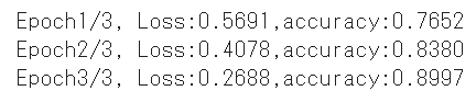
    print(f'Epoch {epoch + 1}/{epochs}, Loss: {avg_loss:.4f}, Accuracy: {accuracy:.4f}')

学習結果と精度の結果が出力されました。

テキストの感情分析

# モデルを評価モードに切り替え
model.eval()

# 新しいテキストで感情分析
new_text = 'This summer is long! Too hot!'
new_input_ids, new_attention_mask = tokenize_to_text(new_text)
new_outputs = model(new_input_ids, new_attention_mask)
result = torch.argmax(new_outputs.logits, dim=1).tolist()[0]

# 新しい感情分析の結果をキーにマッピングするための逆辞書を作成
reverse_label_mapping = {v: k for k, v in label_mapping.items()}

# resultを使用して感情分析の結果のキーを取得
predicted_emotion = reverse_label_mapping[result]

print("Text:", new_text, "\nPredicted Emotion:", predicted_emotion)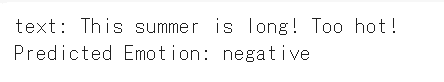

テキストの分析結果

テキストもネガティブと判定をされました。

まとめ

今回の結果から、BERTがRNNよりも高い精度を示しましたが、その一方で実行時間はBERTの方が長くなりました。
具体的には、RNNの実行時間は3分で、BERTの実行時間は1時間でした。BERTの処理がより複雑であるためです。

この学習を通じて、機械学習における前処理の重要性を改めて認識しました。それぞれのモデルが持つ長所と短所を理解し、これからの学習でさらに理解を深めていきたいと思います。

長い間お付き合いいただき、ありがとうございました。