
Photo by
hoho8888
Rを使った主成分分析(2021年8月改訂)

最近、以前書いていた方法ではうまくできなかったので、2021年8月に改定しました。
2021年8月時点で、私のRのバージョンは R version 4.0.3 (2020-10-10) です。Bioconductorも下記サイトで再インストールしました。Bioconductor 3.13です。
https://bioconductor.org
> if (!requireNamespace("BiocManager", quietly = TRUE))
+ install.packages("BiocManager")
> BiocManager::install()
ーーー
メタゲノム、トランスクリプトーム、メタボロームなどのオミックスデータのサンプル間の比較でよく用いられる主成分分析の方法。
まずは、準備として、Rのメニューバーの”パッケージとデータ”>"パッケージインストーラ"で"ggplot2" と "rgl" パッケージをインストール。
”meshr" もインストールしておきましょう。
下記のコマンドでもインストールできます。
> BiocManager::install("meshr")例えば、図のようなデータが与えられたとき、
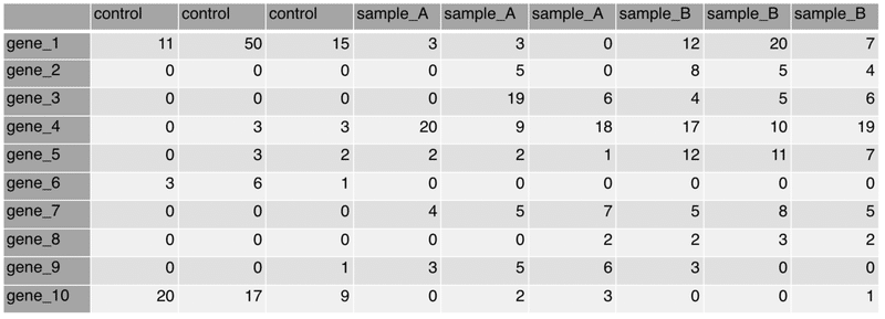
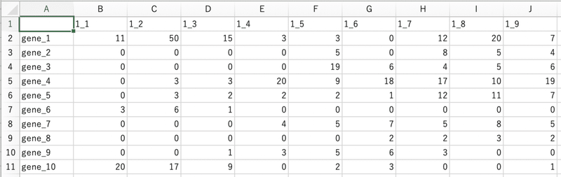
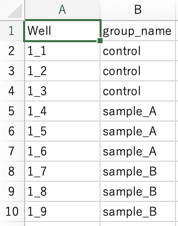
DataのファイルとGroupのファイルを以下のように作成し、csvファイルとして保存します。
Dataファイル;table.csv
Groupファイル;group.csv
ファイルを置いてある作業ディレクトリ、ここではデスクトップへ移動。
> setwd("~/Desktop")
DataとGroupの2つのファイルを読み込み。
> group<-read.csv("group.csv", header=T)
> data<-read.csv("table.csv", row.name=1, header=T)
確認
> group
 Well group_name
1  1_1    control
2  1_2    control
3  1_3    control
4  1_4   sample_A
5  1_5   sample_A
6  1_6   sample_A
7  1_7   sample_B
8  1_8   sample_B
9  1_9   sample_B

> data
       X1_1 X1_2 X1_3 X1_4 X1_5 X1_6 X1_7 X1_8 X1_9
gene_1    11   50   15    3    3    0   12   20    7
gene_2     0    0    0    0    5    0    8    5    4
gene_3     0    0    0    0   19    6    4    5    6
gene_4     0    3    3   20    9   18   17   10   19
gene_5     0    3    2    2    2    1   12   11    7
gene_6     3    6    1    0    0    0    0    0    0
gene_7     0    0    0    4    5    7    5    8    5
gene_8     0    0    0    0    0    2    2    3    2
gene_9     0    0    1    3    5    6    3    0    0
gene_10   20   17    9    0    2    3    0    0    1
データファイルの行列変換
> data2<-t(data)
> data2
    gene_1 gene_2 gene_3 gene_4 gene_5 gene_6 gene_7 gene_8 gene_9 gene_10
X1_1     11      0      0      0      0      3      0      0      0      20
X1_2     50      0      0      3      3      6      0      0      0      17
X1_3     15      0      0      3      2      1      0      0      1       9
X1_4      3      0      0     20      2      0      4      0      3       0
X1_5      3      5     19      9      2      0      5      0      5       2
X1_6      0      0      6     18      1      0      7      2      6       3
X1_7     12      8      4     17     12      0      5      2      3       0
X1_8     20      5      5     10     11      0      8      3      0       0
X1_9      7      4      6     19      7      0      5      2      0       1
Data2のファイルにWell列を足して、groupファイルのWell列を記入。
> data3 <- data.frame(data2, Well=sub("X", "", rownames(data2)))
> colnames(group)[1]<-"Well"
> data3
    gene_1 gene_2 gene_3 gene_4 gene_5 gene_6 gene_7 gene_8 gene_9 gene_10 Well
X1_1     11      0      0      0      0      3      0      0      0      20  1_1
X1_2     50      0      0      3      3      6      0      0      0      17  1_2
X1_3     15      0      0      3      2      1      0      0      1       9  1_3
X1_4      3      0      0     20      2      0      4      0      3       0  1_4
X1_5      3      5     19      9      2      0      5      0      5       2  1_5
X1_6      0      0      6     18      1      0      7      2      6       3  1_6
X1_7     12      8      4     17     12      0      5      2      3       0  1_7
X1_8     20      5      5     10     11      0      8      3      0       0  1_8
X1_9      7      4      6     19      7      0      5      2      0       1  1_9
Groupとdata3のファイルを"Well”でマージ。
> data4 <- merge(group, data3, by ="Well")
> data4
 Well group_name gene_1 gene_2 gene_3 gene_4 gene_5 gene_6 gene_7 gene_8 gene_9 gene_10
1  1_1    control     11      0      0      0      0      3      0      0      0      20
2  1_2    control     50      0      0      3      3      6      0      0      0      17
3  1_3    control     15      0      0      3      2      1      0      0      1       9
4  1_4   sample_A      3      0      0     20      2      0      4      0      3       0
5  1_5   sample_A      3      5     19      9      2      0      5      0      5       2
6  1_6   sample_A      0      0      6     18      1      0      7      2      6       3
7  1_7   sample_B     12      8      4     17     12      0      5      2      3       0
8  1_8   sample_B     20      5      5     10     11      0      8      3      0       0
9  1_9   sample_B      7      4      6     19      7      0      5      2      0       1
Label用のファイルを作成
> Label <- data.frame(group_name=data4$group_name, Color=NA, Name=NA)
> Label$Color[which(Label$group_name=="sample_A")]<- rgb(1, 0, 0, 0.5)
> Label$Color[which(Label$group_name=="sample_B")]<- rgb(0, 1, 0, 0.5)
> Label$Color[which(Label$group_name=="control")]<- rgb(0, 0, 0, 0.5)
> Label$Name[which(Label$group_name=="sample_A")]<- "A"
> Label$Name[which(Label$group_name=="sample_B")]<- "B"
> Label$Name[which(Label$group_name=="control")]<- "control"
> Label
 group_name     Color     Name
1    control #00000080  control
2    control #00000080  control
3    control #00000080  control
4   sample_A #FF000080  A
5   sample_A #FF000080  A
6   sample_A #FF000080  A
7   sample_B #00FF0080  B
8   sample_B #00FF0080  B
9   sample_B #00FF0080  B
Data4から必要な部分だけ取り出して、行列変換。
> data5<-t(data4[,3:ncol(data4)])
> data5
       [,1] [,2] [,3] [,4] [,5] [,6] [,7] [,8] [,9]
gene_1    11   50   15    3    3    0   12   20    7
gene_2     0    0    0    0    5    0    8    5    4
gene_3     0    0    0    0   19    6    4    5    6
gene_4     0    3    3   20    9   18   17   10   19
gene_5     0    3    2    2    2    1   12   11    7
gene_6     3    6    1    0    0    0    0    0    0
gene_7     0    0    0    4    5    7    5    8    5
gene_8     0    0    0    0    0    2    2    3    2
gene_9     0    0    1    3    5    6    3    0    0
gene_10   20   17    9    0    2    3    0    0    1
PCA計算
> pca <- prcomp(data5, scale = TRUE)
> summary(pca)
Importance of components:
                         PC1    PC2    PC3     PC4     PC5     PC6     PC7     PC8     PC9
Standard deviation     1.9584 1.7679 0.9906 0.89327 0.39786 0.24857 0.18769 0.06639 0.01529
Proportion of Variance 0.4262 0.3473 0.1090 0.08866 0.01759 0.00687 0.00391 0.00049 0.00003
Cumulative Proportion  0.4262 0.7734 0.8825 0.97112 0.98871 0.99557 0.99948 0.99997 1.00000
3d グラフを描いて回してみる。
> library("rgl")
> plot3d(pca$rotation[, 1:3], xlab="PC1", ylab="PC2", zlab="PC3", col=Label$Color)
2Dで論文用に図を描画。
> library(maptools)
> plot(pca$rotation[,1],pca$rotation[,2], col=Label$Color, pch=19, cex =3)
> pointLabel(pca$rotation[,1],pca$rotation[,2], labels=Label$Name)
保存
ラベルなし
> tiff(filename="test_PCA.tiff")
> plot(pca$rotation[,1],pca$rotation[,2], col=Label$Color, pch=19, cex =3)
> dev.off()
quartz
2 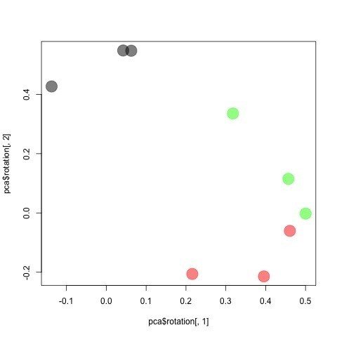
ラベルあり
> tiff(filename="test_PCA.tiff")
> plot(pca$rotation[,1],pca$rotation[,2], col=Label$Color, pch=19, cex =3)
> pointLabel(pca$rotation[,1],pca$rotation[,2], labels=Label$Name)
> dev.off()
quartz
2 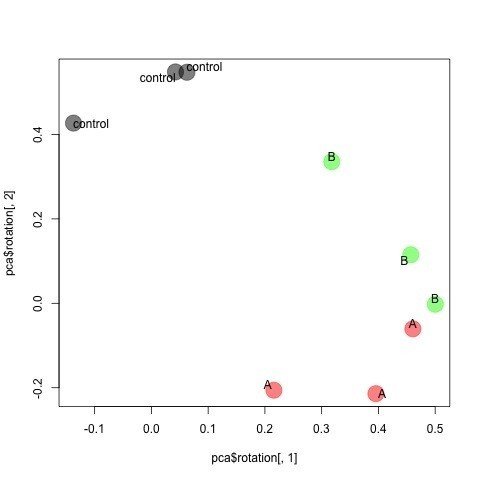
この記事が気に入ったらサポートをしてみませんか?